It turns out that the Smith chart is still the basic tool for determining the impedance of a transmission line. When dealing with the practical application of the RF system, there are always some very difficult tasks, and matching one of the different impedances of the cascading circuits is one of them. In general, the circuits that need to be matched include the match between the antenna and the low noise amplifier (LNA), the match between the power amplifier output (RFOUT) and the antenna, and the match between the LNA/VCO output and the mixer input. The purpose of matching is to ensure that the signal or energy is effectively transferred from the "signal source" to the "load". At the high frequency end, parasitic components (such as inductance on the wire, capacitance between the layers, and resistance of the conductor) have a significant, unpredictable effect on the matching network. When the frequency is above tens of megahertz, the theoretical calculations and simulations are far from satisfactory. In order to get the appropriate final results, the RF test in the laboratory must be considered and properly tuned. The calculated value is used to determine the type of structure of the circuit and the corresponding target component value. There are many ways to match impedance, including
Computer Simulation: Because this type of software is designed for different functions and not just for impedance matching, it is more complicated to use. Designers must be familiar with entering large amounts of data in the correct format. Designers also need the skills to find useful data from a large number of output results. In addition, circuit emulation software cannot be pre-installed on a computer unless the computer is specifically designed for this purpose.
Manual calculation: This is an extremely cumbersome method because it requires a longer ("several kilometers") calculation formula and the processed data is mostly complex.
Experience: This method can only be used by people who have worked in the RF field for many years. In short, it is only suitable for experienced experts.
Smith Chart: This article will focus on the content.

The chart was invented in 1939 by Phillip Smith, who worked at RCA in the United States. Smith once said, "When I can use the slide rule, I am interested in graphically expressing the mathematical relationship." The basics of the Smith chart are the following formulas.  The Γ in the middle represents the reflection coefficient of the line, that is, S11 in the S-parameter (S-parameter), and ZL is the normalized load value, that is, ZL / Z0. Among them, ZL is the load value of the line itself, and Z0 is the characteristic impedance (intrinsic impedance) value of the transmission line, usually 50Ω is used. To put it simply: just like mathematics, look up and know the value of the reflection coefficient. 2. Why? We don't know now, how did Mr. Smith think of the inspiration for the "Smith Chart" representation? Many students read Smith's original picture, remembering hardbacks, and not asking for it. In fact, there is no attempt to figure out the original intention of Mr. Smith. I personally speculate: Is it inspired by Riemann's geometry to give a plane coordinate system to the "bend". I am expressing the process of this "bending", you understand, the meaning of this figure. (The coordinate system can bend, people try not to "bend"; if it has been bent, I express blessing) Now, I will show you the bend. The world map is actually a process of using a plane to represent a sphere. This process is a "straight".

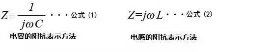
The original image of Smith, ingenious, is to use a circle to represent an infinite plane. 2.1. First, let us first understand the plane of "infinity." First of all, let's review the impedance of the ideal resistor, capacitor, and inductor. In circuits with resistors, inductors, and capacitors, the blocking effect on the current in the circuit is called impedance. The impedance is usually represented by Z. It is a complex number. It is actually called a resistor. It is called a reactance. The blocking effect of the capacitor on the alternating current in the circuit is called capacitive reactance. The inductance is a hindrance to the alternating current in the circuit. The resistance of capacitors and inductors to alternating current in the circuit is collectively referred to as reactance. The unit of impedance is ohms. R, resistance: In the same circuit, the current through a conductor is proportional to the voltage across the conductor and inversely proportional to the resistance of the conductor. This is Ohm's law. Standard style:  . (The ideal resistance is a real number and does not involve the concept of a complex number). If we introduce the concept of complex numbers in mathematics, we can express the resistance, inductance, and capacitance in the same form of complex impedance. Both: the resistance is still the real number R (the real part of the complex impedance), and the capacitance and inductance are represented by imaginary numbers, respectively:
Z= R+i( ωL–1/(ωC)) Description: The load is the three types of complex of the resistance, inductance and capacitance of the capacitor. After compounding, it is called “impedanceâ€. It is written as a mathematical formula: impedance Z = R + i (ωL - 1 / (ωC)). Where R is the resistance, ωL is the inductive reactance, and 1/(ωC) is the capacitive reactance. (1) If (ωL–1/ωC) > 0, it is called “inductive loadâ€; (2) Conversely, if (ωL–1/ωC) < 0 is called “capacitive loadâ€. Let's take a closer look at the impedance equation, which is no longer a real number. It becomes a complex number because of the presence of capacitors and inductors.
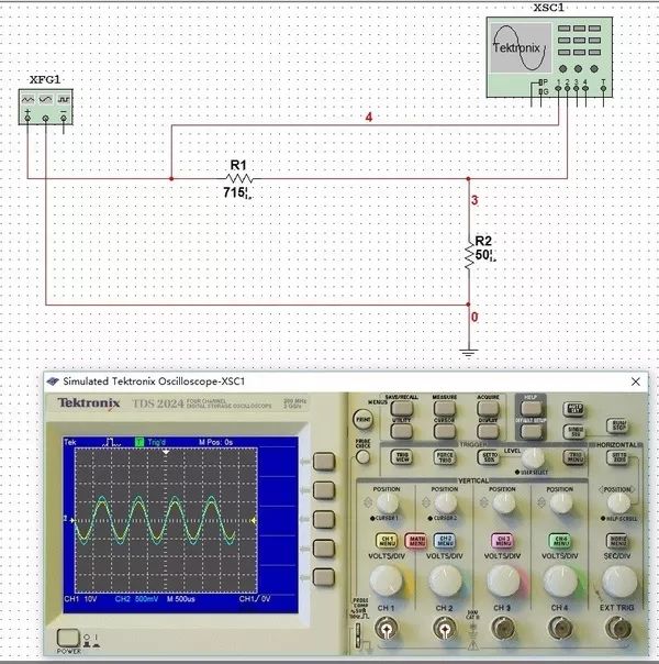
If there is only a resistor in the circuit, it only affects the amplitude change.

From the above figure, we know that the amplitude of the sine wave has changed, and at the same time, the phase has also changed, and the frequency characteristics also change. Therefore, in the process of calculation, we need to consider the real part, but also need to consider the imaginary part. We can represent any complex number in a complex plane with the real part as the x-axis and the imaginary part as the y-axis. Our impedance, no matter how many resistors, capacitors, inductors are connected in series, in parallel, can be represented in a complex plane.

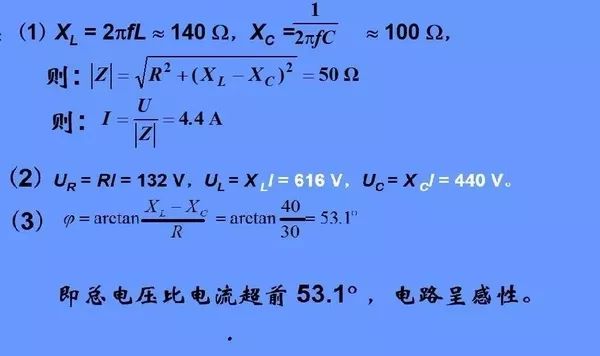
In the RLC series circuit, the AC supply voltage U = 220 V, frequency f = 50 Hz, R = 30 Ω, L = 445 mH, C = 32 mF.

In the above figure, we see the superposition of several vectors, the final impedance in the complex plane, falling in the blue dot position. Therefore, the calculation result of any one impedance can be placed at the corresponding position of this complex plane. The various impedances make up this infinite plane. 2.2. When the reflection formula signal propagates forward along the transmission line, a transient impedance is felt every moment. This impedance may be the transmission line itself, or it may be midway or other components at the end. For a signal, it doesn't distinguish exactly what it is, and the signal only senses the impedance. If the impedance felt by the signal is constant, then it will propagate forward normally, as long as the perceived impedance changes, no matter what it is caused (may be resistance, capacitance, inductance, via, PCB corner encountered in the middle) , connector), the signal will be reflected.

The tide of the Qiantang River is that the width of the channel causes a reflection, which is not consistent with the impedance in the circuit, resulting in signal reflection, which can be analogous. The energy of the reflection gathers together, causing an overshoot. Maybe this metaphor is not appropriate, but it is quite image.

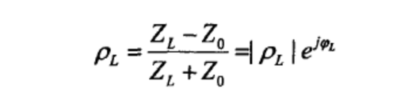
So how much is reflected back to the starting point of the transmission line? An important measure of the amount of signal reflection is the reflection coefficient, which is the ratio of the reflected voltage to the original transmitted signal voltage. The reflection coefficient is defined as:
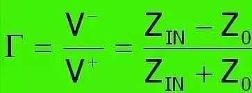
Where: Z0 is the impedance before the change, and ZIN is the impedance after the change. Assuming that the characteristic impedance of the PCB line is 50 ohms, a 100 ohm chip resistor is encountered during transmission. The effect of the parasitic capacitance inductance is not considered for the time being. The resistance is regarded as the ideal pure resistance, and the reflection coefficient is: 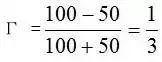 One third of the signal is reflected back to the source. If the voltage of the transmitted signal is 3.3V, the reflected voltage is 1.1V. The reflection of a purely resistive load is the basis for studying the reflection phenomenon. The change of the resistive load is nothing more than the following four cases: the finite value of the impedance increases, the finite value decreases, the open circuit (the impedance becomes infinite), the short circuit (the impedance suddenly becomes 0) ).

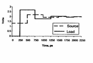
The initial voltage is the source voltage Vs (2V) divided by Zs (25 ohms) and transmission line impedance (50 ohms). The subsequent reflectivity of Vinitial=1.33V is calculated according to the reflection coefficient formula.
The reflectivity at the source is calculated from the source impedance (25 ohms) and the transmission line impedance (50 ohms) according to the reflection coefficient formula to -0.33; the terminal reflectivity is based on the termination impedance (infinity) and the transmission line impedance (50 ohms). The reflection coefficient formula is calculated as 1; we obtain this waveform by superimposing on the initial pulse waveform according to the amplitude and delay of each reflection, which is why the impedance mismatch causes poor signal integrity.
Then we make an important assumption! In order to reduce the number of unknown parameters, it is possible to cure a parameter that often occurs and is often used in applications. Here Z0 (characteristic impedance) is usually a constant and is a real number, which is a commonly used normalized standard value such as 50 Ω, 75 Ω, 100 Ω, and 600 Ω. Assuming Z0 is certain, it is 50 ohms. (Why is it 50 ohms, it is not listed here; of course, other assumptions can be made to make it easier to understand. We will definitely decide to die 50Ω). Then, according to the reflection formula, we get an important conclusion:

We portray the correspondence to the "complex plane" we just said. So we can define the normalized load impedance: 
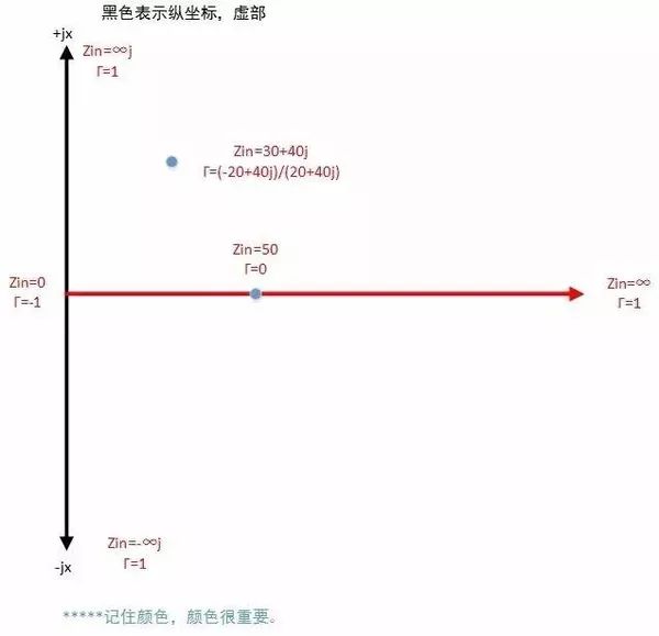
Ok, we are in the complex plane, forget Zin, just remember z (lowercase) and the reflection coefficient "Γ". Preparations are all done, below we are ready to "bend" 2.3 掰 bend
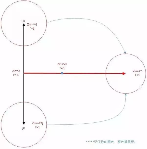
In the complex plane, there are three points, and the reflection coefficient is 1, which is the infinity of the abscissa and the positive and negative infinity of the ordinate. One day in history, Mr. Smith, if you have the help of God, bend the black line and pinch the points marked in the three red circles in the above picture. Bent, bent

Round, round.

Perfect circle:
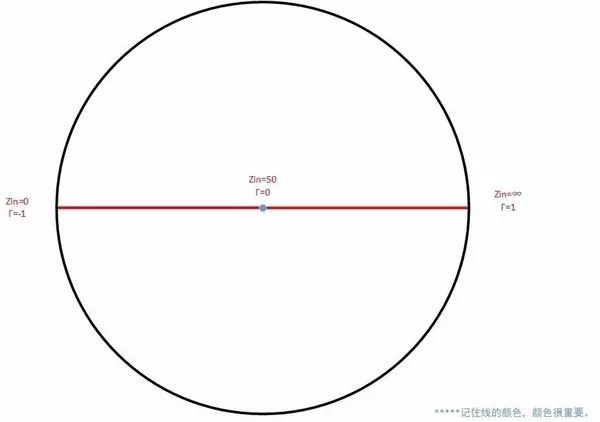
Although the infinity plane becomes a circle, the red line is still a red line, and the black line is still a black line. At the same time, we added three lines to the original complex plane, which also curved as the plane closed.
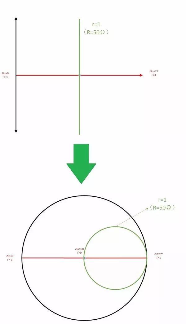
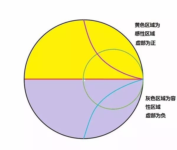
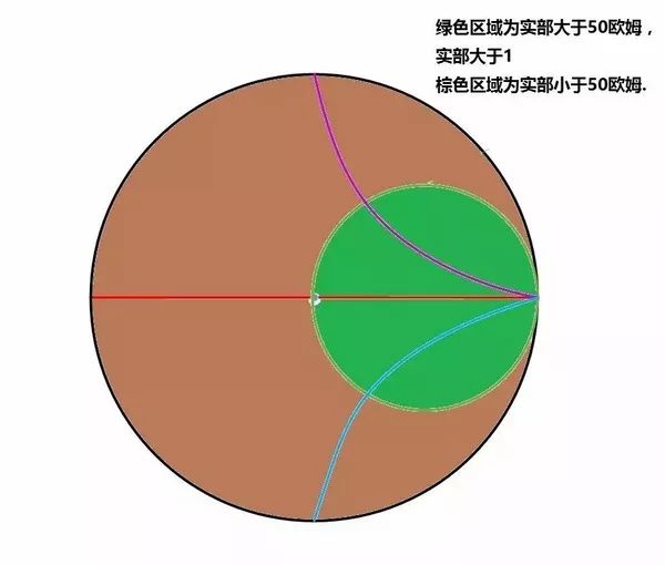
The impedance of the black line has a characteristic: the real part is 0; (resistance is 0) the impedance of the red line has a characteristic: the imaginary part is 0; (inductance, capacitance is 0) the impedance on the green line There is a characteristic: the real part is 1; (resistance is 50 ohms) The impedance of the purple line has a characteristic: the imaginary part is -1; the impedance of the blue line has a characteristic: the imaginary part is 1;

The impedance characteristics of the line, we are moving from the complex plane to the original image of Smith, so the characteristics follow the color and the characteristics are unchanged.
The lower semicircle is the same division as the working circle.

Because the Smith chart is a graph-based solution, the accuracy of the results is directly dependent on the accuracy of the graph. The following is an example of an RF application represented by a Smith chart: Example: The known characteristic impedance is 50Ω and the load impedance is as follows:
| Z1= 100 + j50Ω | Z2= 75 - j100Ω | Z3= j200Ω | Z4= 150Ω |
| Z5= ∞ (an open circuit) | Z6= 0 (a short circuit) | Z7= 50Ω | Z8= 184 - j900Ω |
Normalize the above values ​​and mark them in the circle chart (see Figure 5):
| Z1= 2 + j | Z2= 1.5 - j2 | Z3= j4 | Z4= 3 |
| Z5= 8 | Z6= 0 | Z7= 1 | Z8= 3.68 - j18 |
We can't see the picture above. If it is "series", we can first determine the real part on the clear Smith original image (the red line is found, the horizontal coordinate of the original complex plane), and then according to the imaginary part of the imaginary part, slide along the arc to find our corresponding Impedance. (Ignore the green line in the figure below)

The reflection coefficient Γ can now be solved directly from the circle diagram. We can either directly read the value of the reflection coefficient by Cartesian coordinates or read the value of the reflection coefficient by polar coordinates. The rectangular coordinates plot the impedance point (the intersection of the equal impedance circle and the equal reactance circle). As long as they are projected on the horizontal and vertical axes of the Cartesian coordinate, the real part Γr and the imaginary part åå°„i of the reflection coefficient are obtained. 6). There may be eight cases in this example. The corresponding reflection coefficient can be directly obtained on the Smith chart shown in Figure 6:
| Γ1= 0.4 + 0.2j | Γ2= 0.51 - 0.4j | Γ3= 0.875 + 0.48j | Γ4= 0.5 |
| Γ5= 1 | Γ6= -1 | Γ7= 0 | Γ8= 0.96 - 0.1j |
Direct reading of the real and imaginary polar coordinates of the reflection coefficient Γ from the XY axis
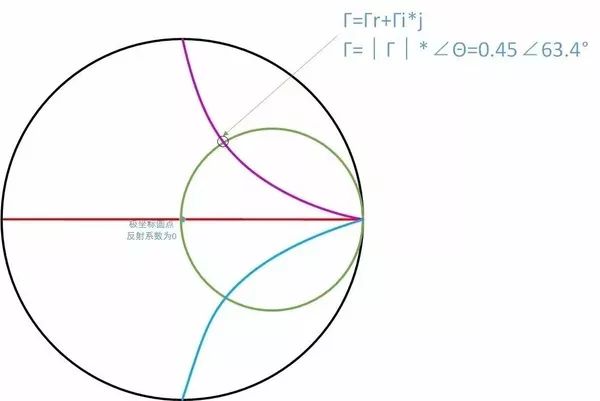
Polar coordinates, what is the use? Very useful, this is actually the purpose of Smith's original picture. 2.4 Red Camp VS Green Camp

We have just noticed that the original picture of Smith, in addition to the red curve, is the red world from the complex plane of the impedance. At the same time, in the figure, there are green curves, which are generated from the admittance complex plane and the bend. The process is the same as the one just after. So what is the use of this green admittance? Parallel circuits, using admittance calculations, we will be very convenient. At the same time, in the original Smith chart, we can use the green curve of the admittance to query, it will be very convenient.
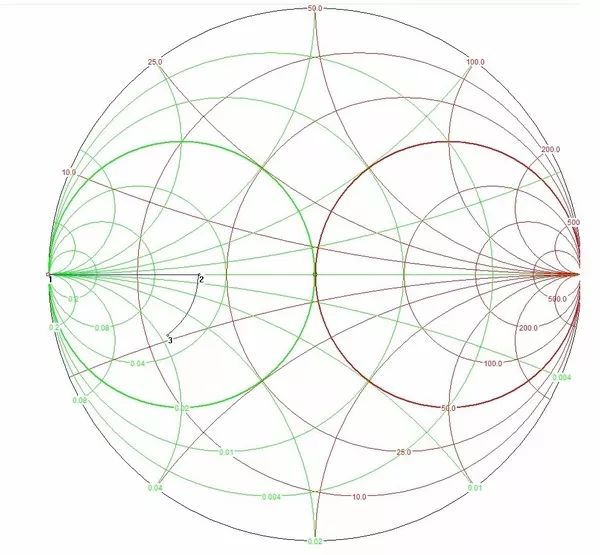

As shown in the figure, a capacitor is connected in parallel, and the corresponding normalized impedance and reflection coefficient can be quickly queried through the green curve. 3. What are you doing? Explain and introduce the long paragraph of the Smith chart, don't forget what we want to do. We actually hope that the circuit reflection coefficient we design is closer to 0. But what kind of circuit is a qualified circuit? The reflection coefficient cannot be ideally zero, so what are our requirements for the reflection coefficient? We want the absolute value of the reflection coefficient to be less than 1/3, that is, the reflection coefficient falls into the blue area of ​​the Smith chart (as shown below).

What is the characteristic of this blue ball? In fact, we have clearly found out through the value of Smith's original image. On the central axis, which is the red line previously mentioned, it is 25 ohms and 100 ohms respectively. That is: Zin is in the area between 1/2 Zo and 2 times Zo.
That is, we target the blue area and think that the reflection coefficient is acceptable.
Instruction Manual
1. Features
Clock display, 10 sets of adjustable timed power control, randomized power control, manual switch and optional DST setup.
2. First time charging
This timer contains a rechargeable battery. It is normal that the new/old model runs out of battery if it wasn`t being charged for a long period of time. In this case, the screen will not turn on.
To charge : simply plug the timer to a power outlet. The charging time should take at least 15 minutes.
If the screen doesn`t light up or displays garbled characters, simply reboot the system by pressing the [RESET" button.
3. Set clock
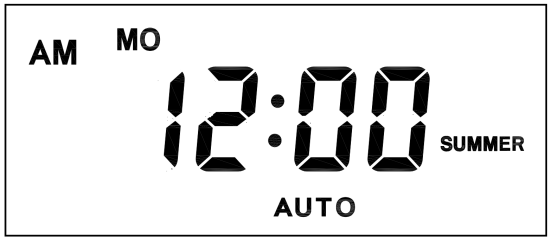
Hold [CLOCK" button and [WEEK" button to adjust week.
Hold [CLOCK" button and [HOUR" button to adjust hour.
Hold [CLOCK" button and [MINUTE" button to adjust minute.
Hold [CLOCK" button and [TIMER" button to select 12 hour/24 hour display.
Hold [CLOCK" button and [ON/AUTO/OFF" button to enable/disable DST (daylight-saving-time).
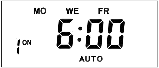
4. Set timer
Press [TIMER" button, select and set timer. Setting rotation : 1on, 1off, 2on, 2off, ...... , 10on, 10off.
Press [HOUR" button to set hour for timer.
Press [MIN" button to set minute for timer.
Press [WEEK" button to set weekday for timer. Multiple weekdays can be selected. ex: if selected [MO", the timer will only apply on every Monday; if selected [ MO, WE, FR", the timer will apply on every Monday, Wednesday and Friday.
Press [RES/RCL" button to cancel the selected on or off timer. The screen will show "-- -- : -- --" , the timer is canceled.
Press [RES/RCL" button again to reactivate the timer.

When timers are set, press [CLOCK" to quit timer setting and return to clock.
5. Random function

Press [RANDOM" button to activate random function, press again to cancel function.
System only runs random function when [AUTO" is on.
Random function will automatically start the timer from 2 to 32 minutes after the setting.
ex : if timer 1on was set to 19:30 with the random function on, the timer will activate randomly between 19:33 to 20:03.
if timer 1off was set to 23:00 with the random function on, the timer will activate randomly between 23:02 to 23:32.
To avoid overlapping, make sure to leave a minimum of 31 minutes gap between different sets of timer.
6. Manual control
Displayed features:
ON : socket turns on.
OFF : socket turns off.
AUTO : socket turns on/off automatically via timer.
Manual ON setting
Press [ON/AUTO/OFF" button to switch from [AUTO" to [ON".
This mode allows socket of the device to power up. Power indicator will light up.
Manual OFF setting
Press [ON/AUTO/OFF" button to switch from [AUTO" to [OFF".
This mode turns socket of the device off. Power indicators will turn off.
7. Electrical parameters
Operating voltage : 230VAC
Battery : NiMh 1.2V
Power consumption : < 0.9W
Response time : 1 minute
Power output : 230VAC/16A/3680W
Q&A
Q: Why won`t my timer turn on?
A: It`s out of battery, you can charge the timer by plugging onto any power outlet. Charge the device for at least 15 minutes. Then press [RESET " button to reset the device.
Q: Can I set seconds of the timer?
A: No, the smallest time unit is minute.
Q: Does my timer keeps old settings without being plugged onto a power outlet?
A: Yes, the timer has an internal battery, it allows the timer to save settings without a power outlet.
Q: Is the battery rechargeable?
A: Yes, the battery is rechargeable. We recommend to charge it for 4 hours so the battery is fully charged.
Q: Does the timer needs internet connection?
A: The timer does not need internet.
Q: Does the screen have back light function?
A: It doesn`t support back light.
Digital Timer Socket, Timing Switch Socket, Electronic Timer Socket, Timer Socket
NINGBO COWELL ELECTRONICS & TECHNOLOGY CO., LTD , https://www.cowellsockets.com