Machine Learning: Introduction to Random Gradient Descent and Batch Gradient Descent Algorithm

StochasTIc gradient descent

Batch gradient descent

Gradient descent (GD) is a common method to minimize the risk function and loss function. Stochastic gradient descent and batch gradient descent are two kinds of iterative solution ideas. The following two aspects are analyzed from the perspective of formula and implementation. Written wrong, I hope the netizens correct.

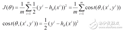
The following h(x) is the function to be fitted, the J(theta) loss function, theta is the parameter, and the value to be solved iteratively, theta solves the function h(theta) that is finally fitted. Where m is the number of records in the training set and j is the number of parameters.

1. The solution to the batch gradient reduction is as follows:

(1) Deriving J(theta) to theta to obtain a gradient corresponding to each theta

(2) Since it is necessary to minimize the risk function, each of the theta is updated according to the negative direction of the gradient of each parameter theta

(3) It can be noticed from the above formula that it obtains a global optimal solution, but each step of the iteration uses all the data of the training set. If m is large, then iteration of this method can be imagined. speed! ! So, this introduces another method, the stochastic gradient drops.

2. The solution to the stochastic gradient descent is as follows:

(1) The above risk function can be written as follows. The loss function corresponds to the granularity of each sample in the training set, and the above batch gradient drop corresponds to all training samples:

(2) The loss function of each sample, the partial derivative of theta is obtained to obtain the corresponding gradient to update theta

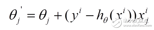
(3) The stochastic gradient descent is iteratively updated by each sample. If the sample size is large (for example, hundreds of thousands), then it is possible to use only tens of thousands or thousands of samples, and theta iteration To the optimal solution, compared to the above batch gradient drop, iteratively requires more than 100,000 training samples, one iteration is impossible to optimize, if iterating 10 times, it needs to traverse the training sample 10 times. However, one problem with SGD is that there is more noise than BGD, so that SGD is not optimized for the entire direction of each iteration.

3. For the linear regression problem above, would the random gradient descent solution be the optimal solution compared to the batch gradient descent?

(1) Batch gradient descent---minimize the loss function of all training samples, so that the final solution is the global optimal solution, that is, the solution parameters are to minimize the risk function.

(2) Stochastic gradient descent---minimize the loss function of each sample, although not the loss function obtained from each iteration is toward the global optimal direction, but the large overall direction is the global optimal solution, the final The result is often near the global optimal solution.

4. Gradient descent is used to find the optimal solution. Which problems can be obtained globally optimally? Which problems may be locally optimal solutions?

For the above linear regression problem, the optimization problem for theta distribution is unimodal, that is, there is only one peak from the top of the graph, so the gradient descent finally finds the global optimal solution. However, for the mulTImodal problem, since there are multiple peak values, it is likely that the final result of the gradient descent is locally optimal.

5. Differences in implementation of random gradients and batch gradients

In the previous blog post, the NMF implementation was taken as an example to list the implementation differences between the two (note: in fact, the code corresponding to Python should be much more intuitive, and you should practice writing more python later!

[java] view plain

// Random gradient drop, update parameters

Digital Printing Graphic Overlay

Digital Printing Graphic Overlay,Membrane Switches Graphic Overlays,Membrane Switch Panels ,Membrane Switch Button

CIXI MEMBRANE SWITCH FACTORY , https://www.cnjunma.com